
A glossy part can look different (reflections) when it turns just a few degrees. On a textured material, normal variability can itself look like a crack, while a real stain disappears under badly angled light. Machine vision inspection automates a quality decision based on images, provided those images make visible a stable difference between a conforming product and a defective one.
On an industrial line, the goal is to apply the same documented, repeatable criterion to every part and keep evidence of each decision. The camera is the first link in a chain that also includes part detection and presentation, image capture under controlled conditions, image analysis, communication with the line control system and recording of the result. Performance depends on the whole chain.
What happens inside a machine vision system?
The cycle starts with an acquisition trigger synchronised with the arrival of the part. The light source creates the contrast and the optics project the scene onto the camera sensor. The resulting image is normalised, cropped or segmented when the process requires it, and then the software applies a set of mathematical rules or a trained model to produce a verdict.
Machine vision systems based on current deep learning models can use many models with different purposes. Classification models, which assign a category to the whole image, such as conforming or defective, are now widely used. Detection models are also very common: they add the position of the defect by means of a bounding region. And of course there are segmentation models, which precisely identify contours pixel by pixel and are very useful for determining the extent and shape of the area affected by a defect. Anomaly detection models complete the picture: they learn what a conforming product looks like and flag whatever departs from it, which makes them especially useful when there are hardly any examples of defects.
The decision can activate a diverter, stop a sequence or send the part for review. For that action to be reliable, the time between capture and result must fit within the cycle time and rate of the production line, as well as the physical distance to the reject point. A correct verdict assigned to the wrong part is still an inspection failure.
A complete station includes mechanical and electrical elements that software cannot replace. Shielding from ambient light, the mechanical stability of mounts and fixtures, and synchronisation all belong to the design of the installation.
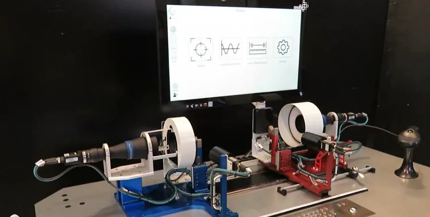
Which defects can be detected and which are out of scope
An industrial machine vision system essentially works when the defect alters an observable optical property. A scratch changes the reflection of a painted panel. In carbon fibre, a discontinuity breaks the apparent regularity of the weave. A cavity or an inclusion changes the visible texture of a sponge. The capture method must reveal the specific anomaly, even though the final outcome is, in every case, a decision made by the quality department.
Conforming products also show variations inherent to the production process of an industrial plant. Fibre orientation, paint gloss or foam porosity can vary within specification. An AI-based machine vision system trained on an overly narrow sample interprets that natural diversity as a defect. Representing acceptable variability is just as important as representing failures, especially with natural or porous materials and reflective finishes.
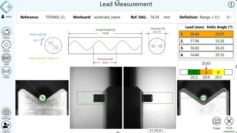
Today, industrial machine vision has a very wide range of uses: the technology serves many purposes, above all in industries where the manufactured product has a high added value that allows a fast return on investment, such as automotive or aerospace.
In general, the most requested applications are:
- 1D & 2D traceability (barcodes, Data Matrix…)
- OCR/OCV
- 2D and 3D vision guidance
- Cosmetic and surface defect inspection
- 2D and 3D metrology.
- Colour measurement
- Bead inspection.
Image capture determines whether the project is feasible
The acquisition hardware of a machine vision system is usually defined in the initial technical feasibility study (Project Qualification), where the most suitable lighting, optics, camera and technologies are evaluated with real parts to maximise the contrast of what has to be detected. The sample set must contain representative conforming parts, defects of varying severity and also parts close to the acceptance limit. The test aims to confirm whether the trace of the defect remains visible when the capture is repeated under the permitted process variations.
Lighting for machine vision systems has also advanced greatly in recent years, mainly thanks to progress in LED technology. LEDs are the most widely used light source today because of the range of geometries they can be packaged in, their excellent controllability, their broad spectral range with many wavelengths and their wide variety of power levels. The lighting system creates much of the contrast required, which then makes processing the acquired image much easier.
The same lighting often does not work for every surface. For example, on a matt surface a frontal light can provide enough contrast, but on a painted panel that same frontal light would create a specular hotspot and hide a scratch. The light source is selected according to how the material and the defect interact.
The viewing direction also plays a part. A camera perpendicular to the surface reduces certain perspective distortions, but it may line up with the reflection of the lighting. On a curved part, no single view keeps the same angle around the whole perimeter. The study then determines whether several cameras provide useful coverage or whether hidden areas remain. Coverage must be stated in terms of inspectable faces and regions, avoiding generic promises about the whole part.
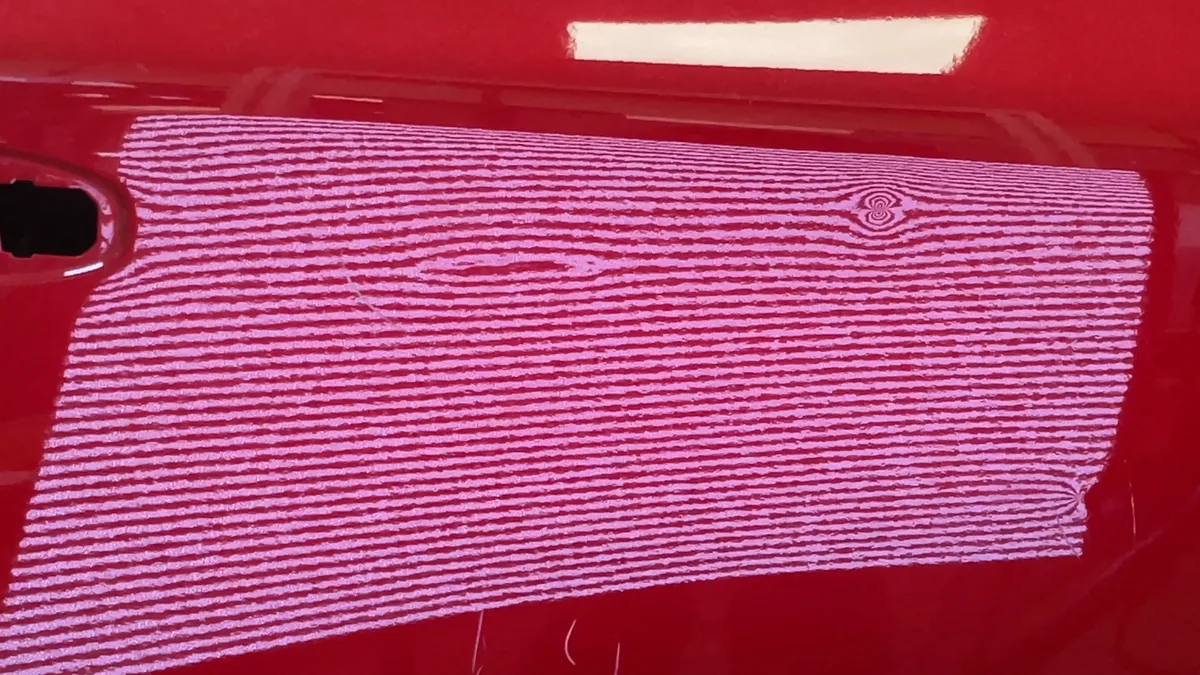
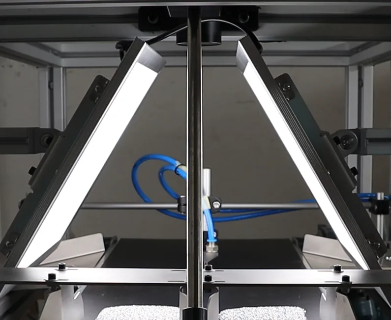
Resolution, on the other hand, refers to the smallest detail that can be distinguished in the field of view. The defect needs to cover enough pixels and keep its contrast once motion and focus are taken into account. A higher-resolution camera increases the amount of information, but optical contrast is still needed to make a defect stand out. Nor can exposure be lengthened freely on a moving line, because motion blur erases precisely the small edges.
The mechanical presentation of the parts to be inspected can introduce another source of uncertainty. A fold in carbon fibre can be told apart from the weave when the part keeps a stable orientation. If it rotates between cycles, the appearance of the fabric changes and the comparison becomes harder. On a sponge, accidental compression alters the pores observed. The sample must reach the camera in the same state in which it was validated, within known position and deformation tolerances. That is why it is crucial to know all the acceptable variability, as far as possible, so that the correct distribution can be estimated right from the validation stage.
The feasibility test ends with a matrix of conditions, not with a single convincing photograph. It records which defects are visible, in which area, with which configuration and under which variations they can no longer be distinguished. If a mark disappears when switching to another conforming batch, or is consistently confused with the normal texture, the test has found a relevant limit. Project feasibility is proven when the separation between OK and NOK parts holds up in real production.
Rules, supervised learning and anomaly detection
Specifically in machine vision systems for cosmetic or surface inspection, algorithms based on explicit rules are a good fit when the feature to be detected can be described by a stable relationship. A contrast threshold can locate a dark stain on a uniform background, and a geometric operation can check that a feature is present. Their behaviour is direct and easy to interpret, but it becomes fragile if the material changes appearance while remaining conforming.
In machine vision systems based on probabilistic models, on the other hand, supervised learning uses labelled images to learn the boundary between classes. It becomes more useful when the defect combines signals that are hard to sum up in a formula, such as texture, local shape and context. Labelling quality sets the practical ceiling of the model: if two specialists classify borderline parts differently, the training set contains an industrial contradiction rather than a software problem.
When defects are scarce (there are not many available for training), anomaly detection models are now used. The model learns the visual distribution of conforming parts and scores deviations, so that parts far removed from what is “normal” can be penalised. This means it can start without an exhaustive catalogue of failures. The challenge arises when a valid variant is new to the model, because visual novelty and a defect are not the same thing, yet both can deviate just as much from the distribution learned as conforming.
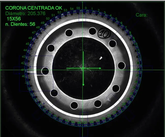
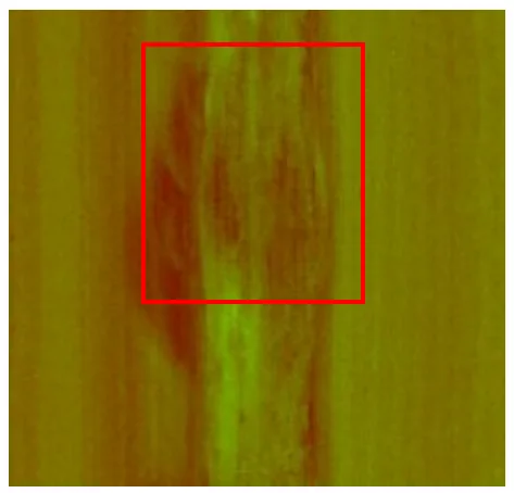
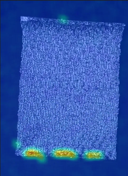
Three approaches: rule-based measurement of a ring gear, a weld defect located by a supervised model and an anomaly model’s heat map on a sponge.
The table positions each approach according to the evidence available and the decision it must produce.
| Approach | Starting evidence | Typical fit | What must be validated |
|---|---|---|---|
| Rules | Samples to set explicit parameters | Stable features with clear separation | Robustness of thresholds to normal variability |
| Supervised learning | Labelled images of the relevant classes | Known defects that must be classified or located | Label consistency, sufficient intra-class diversity and representation of borderline cases |
| Anomaly detection | Representative set of conforming product | Rare or hard-to-anticipate failures | Response to unseen conforming variants |
Data availability is not the only selection criterion. The output the process needs also matters. A classification may be enough to divert the part, whereas a root cause investigation requires the anomaly to be located. If the size of the affected area influences acceptance, segmentation provides a more useful visual basis than a global label.
Hybrid architectures make sense when different areas pose different problems. A stable check can be handled with a rule or a deterministic model, while a finish with a more variable appearance is analysed with a statistical model. Each result then keeps its own validation criterion. The combination must address separate requirements, not pile up algorithms indiscriminately.
Why do false rejects occur and how are they corrected?
A false reject occurs when a conforming part receives a defective verdict. In production, the immediate reaction is usually to move the threshold. That adjustment reduces rejects in the short term, but it also shifts the boundary that protects against real defects. The cause must be found before the sensitivity is changed.
Diagnosis starts with the image. If the supposed anomaly matches a recurring reflection, the source lies in the capture. A mark that moves between cycles points to part presentation or trigger timing. Dirt on an optical protection window, on the other hand, produces fixed patterns that appear on different products. Retraining the model does not fix these errors reliably, because the information source is still degraded; it is more effective to remove the physical cause whenever possible.
The next step is to review how conforming product is represented. A batch of carbon fibre can introduce a valid weave that was not in the original set. On a painted panel, a permitted variation in gloss alters the intensity distribution. If the model only knew a narrow band of appearance, it will flag both as novelty. False rejects clustered by batch or variant reveal gaps in the data. In these cases, retraining once a representative sample of the new acceptable variability has been collected is usually the right course of action.
The third layer is the labelling criterion. A broad category such as “surface defect” can mix rejectable scratches with tolerated cosmetic marks. The model receives visually similar examples with opposite labels and learns an unstable boundary. The review needs the specification and the parts at hand, because a correct label requires the quality department to define the borderline case properly first.
This is where NQInspect, software for detecting anomalies and segmenting defective areas, comes in: it makes it possible to analyse the flagged region and trace the history of results back to the inspected part. Localisation shows whether rejects share an area or an appearance. That evidence guides the review of capture and data, while the conformity decision remains tied to the industrial specification.
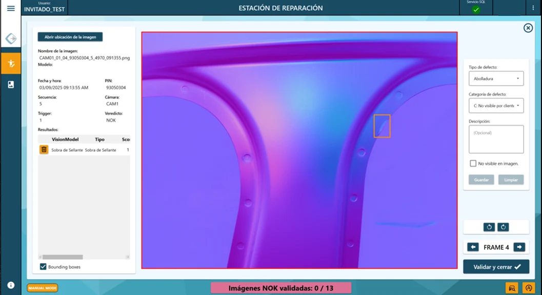
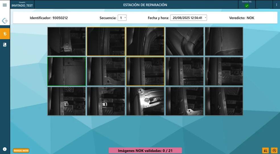
The corrected images form a set of borderline cases. Some extend the conforming variability; others document minor defects that must keep their reject label. These cases are particularly important for learning the boundary. The test set is kept separate from training so that the real effect of each change can be checked. Evaluating with the same images used to tune the system produces false confidence; that is why the sets must always be kept separate.
An overall accuracy rate does not describe the risk either. If good parts are in a large majority, a system can achieve a high percentage while still detecting rare defects poorly. That is why it is important to work with datasets balanced across the different classes. Sensitivity (recall) shows what proportion of known failures is detected, while precision indicates how many alarms actually correspond to a defect. Both metrics must be read together with the population tested and the criterion applied to borderline samples. In other words, neither is a fixed property of the system: precision changes with the proportion of defects in the test population, and sensitivity changes with how difficult the included defects are and how the borderline parts were labelled.
These metrics are calculated from the confusion matrix, a table that cross-references what each part actually is with the system’s verdict:
| Verdict: defective | Verdict: conforming | |
|---|---|---|
| Defective part | True positive (defect detected) | False negative (escape) |
| Conforming part | False positive (false reject) | True negative (conforming part accepted) |
Sensitivity divides the defects detected by all real defects: TP / (TP + FN). Precision divides the defects detected by all alarms: TP / (TP + FP). A third metric, specificity, indicates what proportion of conforming parts is accepted: TN / (TN + FP).
The matrix is not fixed: it depends on the threshold. Lowering it turns escapes into detections, but also turns conforming parts into false rejects; raising it has the opposite effect. Choosing the threshold means deciding which error is more costly, not making a neutral technical adjustment.
Some parts remain close to the threshold even after adjustment. A review zone makes it possible to treat them as uncertain during the stabilisation period, instead of turning a marginal score into an irreversible automatic decision. The reviewed cases feed an exceptions log and show whether disagreement is concentrated in one product family. They are also the examples the model learns most from: prioritising the labelling of the samples the model is unsure about is the core idea of active learning. Explicit uncertainty provides more information than a forced verdict.
How to validate the system before giving it authority over the line
A demonstration with selected images proves that there is a usable pattern. Industrial validation answers a different question: whether the inspection maintains its behaviour under authorised production conditions. The test population must represent the variability the station will encounter, including the accepted extremes.
The plan starts from a reference criterion. The quality department classifies the samples and documents which feature determines the decision. Borderline parts deserve special attention because they concentrate disagreement and drive the threshold setting.
Four tests provide different evidence and must be interpreted together:

- Repeatability with the same sample. The part passes through the station several times under the same recipe. A fluctuating result points to variation in capture, positioning or synchronisation before the classification itself is called into question.
- Reproducibility with authorised production. The test includes representative batches and shifts, as well as approved variants. The aim is to show that the system recognises the differences allowed by the specification as conforming.
- Challenge with defects and borderline parts. The samples cover different defect severities and the area close to the limit. The test shows where separation degrades and avoids reporting performance on obvious cases only.
- Verification of actuation and traceability. Each verdict must act on the part that was captured and leave the correct record. The path to physical rejection is checked, because a timing offset can reject a different part.
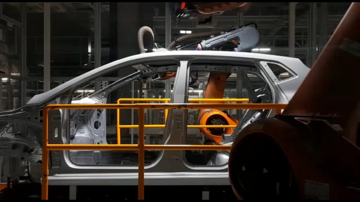
“Shadow mode” adds evidence about in-line behaviour. During this period, the system analyses production without yet taking the final decision, but it stores what that decision would have been. Discrepancies with the current method are reviewed using the image, and the part itself when it is still available. The comparison uncovers variations that the feasibility study carried out in the laboratory may not have reproduced.
Validation also subjects the station to foreseeable operational changes. A restart must not load the wrong recipe. A format change requires the corresponding configuration to be linked, and a loss of communication must leave the system in a known state instead of letting parts through without a result. Behaviour under failure is part of the inspection capability.
The documentation of these inspection systems includes the model version and the relevant acquisition parameters. It also identifies the test set and the results by class, with separate attention to escapes (false negatives) and false rejects (false positives). Later changes are assessed according to their impact.
Changing the camera mount, introducing a visual variant or retraining the model affects different parts of the system and therefore requires the change to be revalidated.
Documented limits protect the interpretation of the result when the line takes on new products.
Traceability and maintenance of the inspection criterion
Traceability starts by linking the verdict to a physical identity. That link can come from the line control system, from the position within a sequence or from association with a batch. The mechanism must prevent a valid acquisition from being assigned to another part, especially when there is a distance between the camera and the reject point.
The record needs the image reference, the result and the active configuration. The timestamp must be synchronised with the other systems involved in the line. When the model produces a score or a segmentation mask, those elements help reconstruct why the alarm was raised. The record describes both the decision and its technical context.
The retention policy is adjusted to the risk, customer requirements and internal needs. Storing every file indiscriminately can make searches harder and consume resources without improving investigations. Rejects provide direct evidence, while a controlled sample of conforming parts makes it possible to check how the normal appearance has evolved. Usefulness depends on the image retaining its traceability.
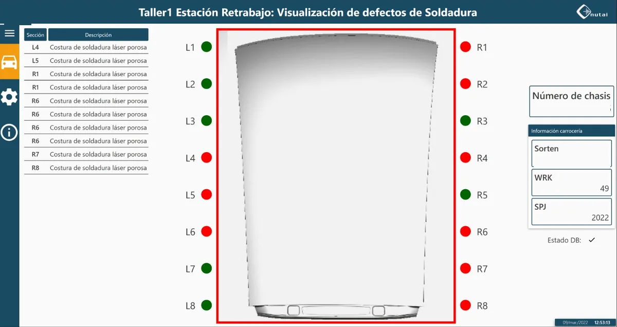
The maintenance phase kicks in when what the camera sees changes. A new supplier can alter the texture while still meeting the functional specification. A change in finish or a new mechanical presentation also has an effect. The alarm rate broken down by variant and context makes it possible to detect these shifts. A localised increase is more diagnostic than the overall reject rate.
Station conditions also change over time. A light can lose stability, the optical protection window can get dirty or a mount can take a knock. Reference images captured under controlled conditions help distinguish optical drift from a change in the product.
Each recipe or model update keeps its reason, the person responsible and the evidence that authorised the change. This makes it possible to reconstruct which configuration inspected a given batch. If a later complaint points to a specific area, the images make it possible to check whether the defect was visible, whether it was scored and what decision it led to. Traceability turns an alarm into a reproducible investigation.
The quality criterion remains an industrial decision
Automation provides repeatability and evidence, but it takes the definition of a defect from the specification agreed with the customer. Disagreement between specialists over the same borderline parts reveals an inadequate specification. Training on that disagreement passes the ambiguity on to the model instead of resolving it.
In a robust implementation, every visual pattern the system detects is tied to its functional or cosmetic consequence. The image makes the difference observable. Engineering and quality determine whether that difference justifies rejection and document the limits of the decision. The system’s authority comes from that validated reference.
When acquisition, criteria and traceability stay aligned, machine vision inspection builds a consistent record of what happened on the line. Each verdict then carries a verifiable explanation in the image and in the configuration that produced it. Consistency comes from technical control of the entire inspection process.


